| . | (2.19) |
| Contents | Previous Chapter | Next Chapter |
In the last chapter the bundling of functions has been introduced, in order to combine and share identical functions as an option for circuit implication.
In a similar form the decomposition of function into subfunctions can be employed for circuit optimization. This is especially true for large combinational circuits, that tend to be confusing because of their high complexity. In most cases these circuits are designed to solve a special problem, so that they do not support general applications.
The circuits should be decomposed into subnets of lower complexity, observing the following criteria for the optimization process:
Definition:
A Boolean Function f(a,b,...) can be decomposed into k Boolean Functions gi(Qi) with i = 1,...,k and Qi ∈ {a,b,...}, if a Boolean Function F(1,...,k) exists, so that:
| . | (2.19) |
Thus multi-stage circuits are formed.
Especially two models of functional decomposition can be distinguished at this point:
The Boolean Function ![]() is called disjunctively decomposable when for all i, j ≦ k and i ≠ j the following applies:
is called disjunctively decomposable when for all i, j ≦ k and i ≠ j the following applies:
| (2.20) |
Figure 2.40: Disjunctive Decomposition of Functions.
A Boolean Function is called iteratively decomposable when a Boolean Function gi(Qi) with i = 1,...,m exists, so that the following applies:
| (2.21) |
| with: | (2.22) |
Example:
Iterative decomposition into 2 functions:
| (2.23) |
Example: Iterative decomposition into 3 functions:
| (2.24) |
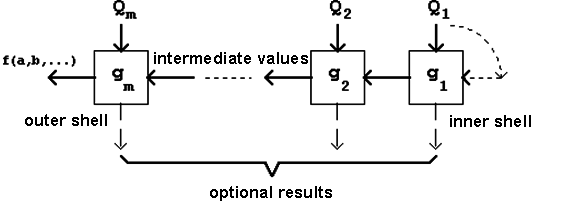
Figure 2.41: Iterative Decomposition of Functions.
The characteristics of functional decomposition will be shown using two important practical examples.
Example 1: Parity Checker
(Disjunctive Decomposition)
Parity checking describes the verification that in a predefined amount of signals the number of 1-signals is even or odd. Accordingly the following is defined:
Figure 2.42: K-Map of the Boolean Function for Odd-Parity-Verification.
This corresponds to the following DNF description (disjunctive normal form) for odd parity verification:
Using the criteria introduced before, the circuit can be evaluated calculating the total gate propagation delay and the total gate input pin count:
| gate delay: | 2 (this is a normal form) |
| pin count: | c = 40 (c = 8*4 + 8: 8 gates with 4 inputs, 1 OR-gate with 8 Inputs) |
It is also possible to describe the Boolean Function for odd-parity verification in a shorter form using the XOR function (Exclusive OR, mathematical symbol: ⊕):
Definition of the XOR-Function:
| (2.25) |
Thus the four-bit parity function can be written as:
| (2.26) |
The function XOR is associative, so that the following is also valid:
| (2.27) |
Functional implementation in a "double rail system":
Figure 2.43: Circuit Implementation of the Parity Checker.
Assessment of the Function:
| gate delay: | 5 (no normal form) |
| pin count: | c = 20 (c = 9*2 + 2*1, see above) |
Example 2: Adder Circuits (Iterative Decomposition)
A circuit for the addition of two dual numbers (adder) can be implemented in a chain structure.
The following truth table distinguishes the adders as
Table 2.9: Truth Table of a Full-Adder; the red colour indicates the Half-Adder.
The red part of the table characterizes the single-stage half-adder which supports the addition of two single-bit dual numbers (i.e. two bits). It determines the result s and the carry bit c.
The single-stage full-adder works just like a half-adder but it includes the carry bit of a previous position. In this case there are two carry bits: the input carry bit
(carry in, cIN)
and the output carry bit (carry out, cOUT).
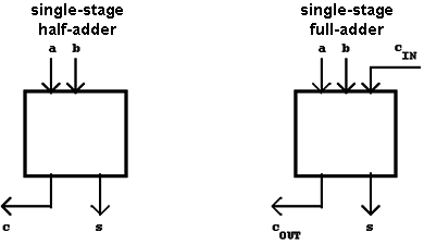
Figure 2.44: Half-Adder and Full-Adder.
The full-adder allows the realization of multi-stage adders:
Chain structure of a n-stage full-adder (ripple adder):
Figure 2.45: n-Stage Full-Adder.
From the above truth table the Boolean Functions s (sum bit) and cOUT (carry out) can be directly derived:
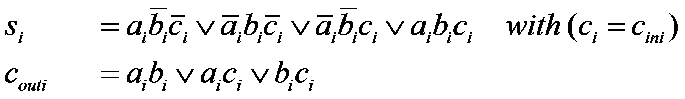 | (2.28) |
Equivalent to this are the following equations:
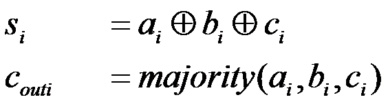 | (2.29) |
Without this iterative decomposition, as shown here, gates of an input width of n + 1 would be necessary to implement an n-stage adder gate. For n > 8 this is not convenient anymore, so that in this case a multi-stage implementation can be considered necessary.
2.10.4 Shannon Decomposition
Another important decomposition method is known as Shannon Decomposition.
Definition: For every Boolean Function f(a,b,...) a non-disjunct decomposition exists, for which the following applies:
| (2.30) |
This functional decomposition method follows directly from the original definition and development of the Karnaugh Diagram. Adding another variable had the consequence that the number of fields is doubled:
When f(a,b) is expanded by an argument c, then one diagram f(a,b) for c=0 and a second diagram f(a,b) for c=1 can be defined. Finally f(a,b) becomes f(a,b,c) by joining the two individual diagrams.
In the Shannon decomposition this process is reversed, the K-Map of the Boolean Function f(a,...,x,...) is cut in half relative to the variable x.
f(a,...,1,...) describes the function in the area x = 1,
f(a,...,0,...) describes the function in the area x = 0.
It follows that when f(a,...,1,...) = 1 or f(a,...,0,...) = 1 the disjunction will also result in f(a,...,x,...) = 1. Only when both subfunctions assume the value '0' the total function too will be f(a,...,x,...) = 0.
The Shannon decomposition can be applied to every Boolean Function. Obviously the functions f(a,...,1,...) and f(a,...,0,...)
that have been defined above, can on their part be divided using the same method.
For a binary (two-element) Boolean Function this results in the following complete decomposition:
 | (2.31) |
Accordingly the decomposition of a three-element Boolean Function can be done:
 | (2.32) |
The numbering of the (not further decomposed) functional terms Si follows as usual the values of the 2-tuples (a,b).
Example:
Defining the Boolean Function f(a,b,c,d) using a K-Map and decomposing it relative to the arguments a and b:
Figure 2.46: Decomposition relative to a and b.
The functional decomposition, graphically shown in the K-Map, can lead to a practical circuit implementation, when the resulting terms Si(c,d) are connected by a hypothetical switch as a function of (a,b) to the output connection Y = f(a,b,c,d).
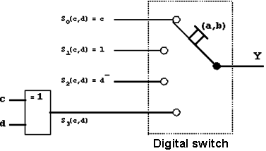
Figure 2.47: Function Decomposition using a Switch.
| Contents | Previous Chapter | Next Chapter |