2 Combinational Circuit Design

2.1 The Karnaugh-Veitch Map (K-Maps)

As an elementary form to represent a Boolean Function the truth table (also called function table) was introduced. That means that a given function can be shown as follows:

Beyond the two function values "0" and "1" two more special cases have to be considered:

• the function value can be chosen arbitrarily ('0' or '1'),
• the input value is irrelevant, but the function value is predefined and fixed.
  

In the truth table both cases can be considered as follows:

Both particular cases have special importance for the optimization of Boolean functions.

This table-oriented procedure to present Boolean functions is precise and very well suited for machine-supported processing. Disadvantage is a fairly unclear formal presentation, in which especially the characteristic properties of a function are difficult to identify.
In order to increase the interpretability of a function, M. Karnaugh and E.W. Veitch suggested a graphical presentation which allows conclusions about the Boolean functions through the verification of special patterns and structures.

Today this presentation is known as a Karnaugh-Veitch Diagram, Karnaugh Map, or simply K-Map. Construction and meaning of this diagram become clear, starting directly from the basic definition of a Boolean function and its set presentation.

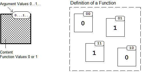
Obviously for an arbitrary Boolean function the following is valid:

• the function's arguments can only have the values "0" or "1",
• the function's value can only be "0" or "1".
  

It follows that a Boolean function f(a,b,...,x) is fully characterized by:

• the arguments a,b,...,x,
• the function values f(a,b,...,x),
• the rule that has to be applied to determine the function value.

Therefore a graphical presentation of the Boolean function can easily be constructed:

Figure 2.3: Developing a Graphical Description of Boolean Functions

In this diagram the argument values define the number of a predefined frame, while the content of the frame reflects the corresponding function value. For a complete description of the function all possible frames are defined and combined into one presentation. This arbitrary frame presentation can be better organized using a systematical definition of the arguments (similar to the definition of axes in a Cartesian coordinate system). Furthermore the isolated boxes will now be connected to a uniform diagram.

For a function with two arguments f(a,b) this leads to the following description:

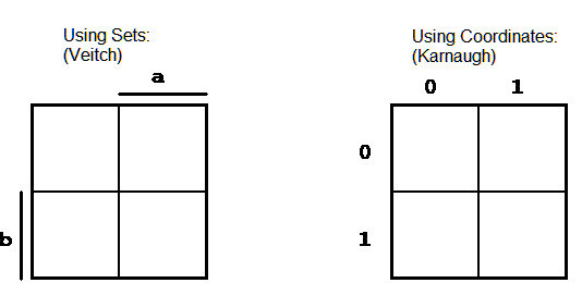
Figure 2.4: Function Diagram according to Veitch and Karnaugh.

To indicate the arguments two usual methods are shown here:

• Set presentation following Veitch, in which the set under the solid line presents a "1" and the remaining set a "0",
• Using 0/1 coordinates (argument values) as suggested by Karnaugh.
  

It is obvious that these two presentation forms are equivalent.

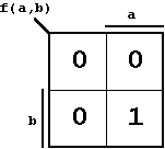
To complete the Diagram (K-Map) the Boolean function under consideration is also indicated.

Example:

Figure 2.5: K-Map (according to Veitch) of the know AND-Function.

Characteristic for the K-Map is also:

• (horizontally or vertically) adjacent fields are different in only one argument value.
  

Graphically this property can be called a "neighbour relation".

Now it is possible to extend the KV Diagrams going beyond two arguments, joining in its most simple form already defined K-Maps to larger areas. Important is that the mentioned "neighbour rule" is maintained during this process.

Example:
Creation of the K-Map for the function f(a,b,c) by adding one more variable and joining the two partial K-Maps (thus doubling the diagram).

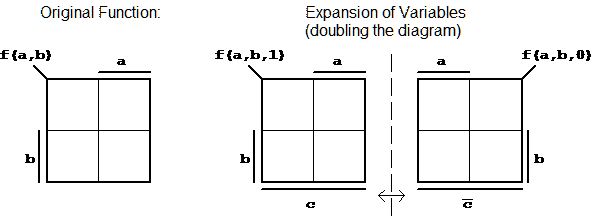
Figure 2.6: Expansion of the K-Map.

Note:
Design Principle for larger Karnaugh Diagrams:

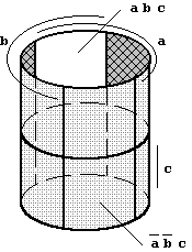
With each addition of another variable the number of function fields will be doubled. When the partial diagrams are joined the neighbour condition has to be observed all the time: neighbouring fields can differ only in one argument value. This "neighbour condition" is also valid at the borders of a Karnaugh diagram. That means that a K-Map - seen three-dimensionally - forms a cylinder (see Figure 2.8).

For a K-Map with four arguments we get the following arrangement:

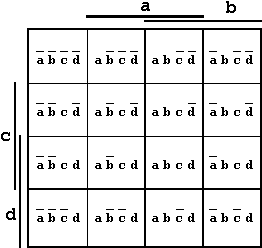
Figure 2.7: K-Map with four Arguments.

The entries shown in each field represent the logical values of the arguments at the corresponding positions.

Figure 2.8: Three-Dimensional Arrangement of a K-Map for three Arguments a,b,c.

Larger K-Maps can be formed following the scheme shown in Figure 2.6, either organizing all arguments in one level (Figure 2.9) or for a better clarity in several levels, thus creating a 3-dimensional structure (Figure 2.10).

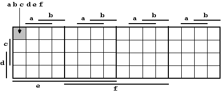
Figure 2.9: Two-Dimensional K-Map for six Variables.

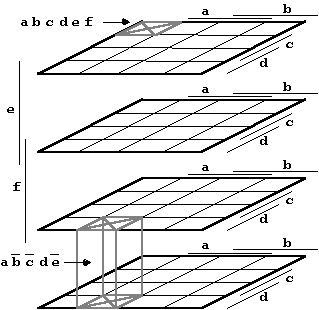
Figure 2.10: Two-Dimensional K-Map for six Variables (shown in three-dimensional form).

Because of their increasing complexity K-Maps are not suitable for the presentation of functions with more than six variables. In these cases other methods have to be applied (see below).

Example:

The Boolean function

Figure 2.11: Boolean Function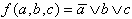

.

The set-oriented view of the Karnaugh Diagram and the correlated development principles will be discussed in a more detailed example. Especially the manipulations and simplifications that are possible with K-Maps make this method a very important design tool.

For the transformation of a Boolean function into a Karnaugh Diagram and the subsequent manipulation the following rules will be observed:

• The set presentation will follow the Veitch convention (using bars).
• The function values correspond to 0- and 1-fields; neighbouring fields with equal values can be combined to sets F0 or F1, respectively (see below for the exact rules).

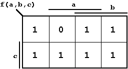
The resulting sets can then be manipulated using the known functions Disjunction, Conjunction, and Complement. These ideas will now be applied to the following Boolean Function f(a,b,c):

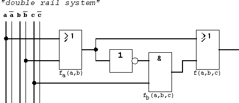
Figure 2.12: Example Function using a "double rail system".

Note:

In this example the input variables a, b, and c are presented in a so-called "double rail system". This means that a variable and it's inverted form are simultaneously available. This also implies an ideal timing behaviour, i.e. that there will not be any delay (see below) between these signals (including the inverted form).

The Karnaugh Diagram of the given Boolean function can be built up step-by-step:

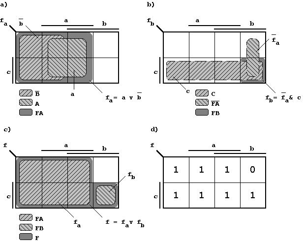
Figure 2.13: Karnaugh Diagrams for the Boolean Function of Figure 2.12.

The K-Maps a) to c) show step-by-step the determination of the Boolean Function f(a,b,c):

Diagram a:

In this diagram the set FA is formed of areas for which f_a(a,b)=1. This set is symmetric to the border of argument c, i.e. it is independent of c! This corresponds to the algebraic expression of the Boolean function

.

Diagram b:

This diagram shows the cut set (conjunction) of the complement of FA and the set C (variable c='1'). The resulting set is FB.

Diagram c:

In diagram c) the sets FA and FB are combined (disjunction) implementing the concluding OR-Function. The final result is set F.

Diagram d:

This diagram reformulates the result c) using the familiar Karnaugh Diagram.

The result of the analysis of this 4-level lattice network is a Boolean Function that produces a '0' under the condition a = c = 0 and b = 1, but generates a '1' in all other cases (see diagram d). This property corresponds to an OR-Function (disjunction).

Obviously the original function can be replaced by a single OR gate without any alteration of the logical behaviour. Furthermore the network will be reduced to one level (1-level), the signal delay is reduced accordingly (to one standard gate delay, see below).

Resulting circuit:

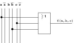
Figure 2.14: Reduced Form of the Circuit in Figure 2.12.